Introduction to Gradient Descent
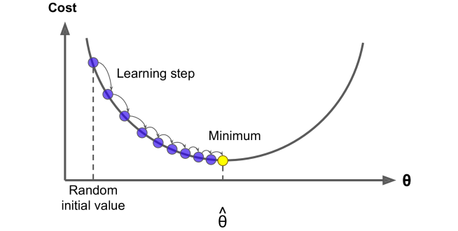
Gradient Descent is a versatile optimization algorithm used to find optimal solutions across various problems. The core concept behind it is to adjust parameters step by step to minimize a given cost function. Imagine being lost in a foggy mountain and only being able to sense the slope of the ground beneath you. To quickly reach the valley, a smart approach would be to move in the direction of the steepest descent. This is essentially how Gradient Descent works: it calculates the gradient of the error function with respect to the parameter vector and moves in the direction where the gradient decreases. When the gradient reaches zero, you’ve found a minimum.
How Gradient Descent Works
In practice, the algorithm starts by initializing parameters with random values, known as random initialization. Then, it iteratively adjusts these values in small steps, each aimed at reducing the cost function, until the algorithm eventually converges to a minimum. A key factor in Gradient Descent is the step size, which is controlled by the learning rate hyperparameter. If the learning rate is set too low, the algorithm will require a large number of iterations to reach convergence, significantly increasing the time it takes to complete. Conversely, if the learning rate is set too high, the algorithm might overshoot the optimal point, causing it to jump back and forth across the minimum or even move further away.
The Importance of Learning Rate
The learning rate is crucial in Gradient Descent. If it’s too small, the process is slow. If it’s too large, the algorithm may not converge. Finding the right balance is key to efficiently reaching the minimum of the cost function. Not all cost functions have smooth, bowl-like shapes. They may contain features like holes, ridges, or plateaus, making it harder to reach the global minimum. If the algorithm starts at a bad point, such as near a local minimum, it might converge to that instead of the global minimum.
Challenges with Gradient Descent
Fortunately, the Mean Squared Error (MSE) cost function for a Linear Regression model is a convex function. This means that for any two points on the curve, the line segment connecting them will not intersect the curve, indicating that there are no local minima — only a single global minimum. Additionally, it is a continuous function with a gradual slope that does not change abruptly. These characteristics ensure that Gradient Descent will reliably get closer to the global minimum, provided you allow sufficient time and maintain an appropriate learning rate.
Feature Scaling and Gradient Descent
The cost function resembles a bowl shape, though it can appear elongated if the features are on significantly different scales. For example, one scenario may show Gradient Descent on a dataset where features are scaled similarly, while another may depict it on a dataset where one feature has much smaller values compared to the others. As illustrated, when features are similarly scaled, the Gradient Descent algorithm moves directly toward the minimum, allowing it to reach the goal quickly. In contrast, when features are not scaled similarly, it initially heads in a direction nearly perpendicular to the global minimum, resulting in a prolonged descent through a nearly flat valley.
Navigating the Parameter Space
Training a model involves searching for a set of parameters that minimizes a cost function based on the training data. This is essentially a search through the model’s parameter space; the more parameters a model has, the higher the dimensionality of this space, making the search more challenging. For instance, locating a needle in a high-dimensional haystack is far more complex than in a three-dimensional one. Fortunately, in the case of Linear Regression, the cost function is convex, meaning the optimal solution can be found at the bottom of the bowl.
Conclusion
Gradient Descent is a cornerstone technique in machine learning, systematically guiding us toward optimal solutions in complex parameter spaces. Its process, comparable to descending a foggy mountain by following the steepest gradient, blends mathematical elegance with practical effectiveness. By carefully tuning the learning rate and applying feature scaling, the algorithm efficiently navigates the cost landscape, avoiding pitfalls like overshooting or stalling. Ultimately, mastering Gradient Descent empowers us to optimize models effectively, making it an essential tool in any data scientist’s toolkit.

