Introduction to Machine Learning for Heart Disease Prediction
In this article, we’ll walk through how to code and experiment with different machine learning algorithms for heart disease prediction. This step-by-step guide will cover data loading, implementing various classification models, and evaluating their performance. Whether you’re a beginner or looking to refine your ML skills, this guide will help you apply multiple algorithms to a real-world dataset in a super simple and straightforward way.
Downloading the Dataset
The first step to create this model is to find and download a dataset. For this project, we will be using the popular “Heart Disease Dataset” csv file on Kaggle. Kaggle is just a platform that has over thousands of different datasets for programmers to use. The link to the dataset can be found here: https://www.kaggle.com/datasets/johnsmith88/heart-disease-dataset.
Loading the Dataset into Colab
Next, we need to load the dataset into an IDE. For this project, I’m using Google Colab. There are two main ways to load the data: uploading the file directly to Colab or uploading to Google Drive and then mounting it in Colab. I highly recommend mounting from Drive. When you upload the file directly to Colab, the dataset is stored in a temporary session, meaning that every time the runtime disconnects, you’ll have to go through the tedious process of re-uploading it.
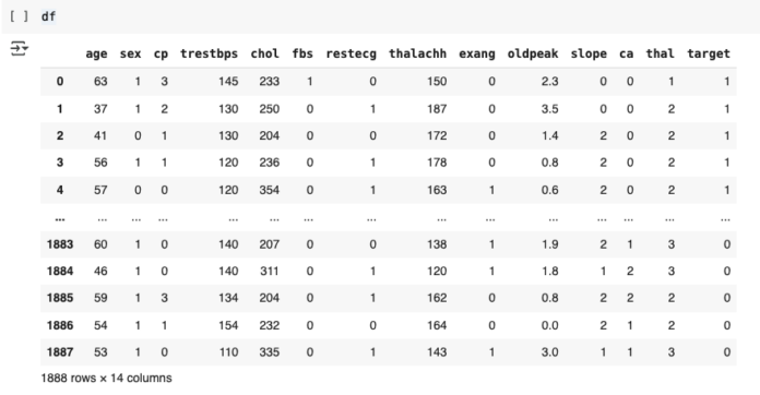
To mount the file in Colab, we first need to import both the Pandas library and the Google Drive module. After running this cell, we will be ready to use Pandas and Google Drive library functions. The drive.mount(“/content/drive”) line allows Colab to access your Google Drive, so that it can actually be mounted. To store the dataset as a Pandas DataFrame, all we have to do is run this following line of code. We set the DataFrame variable as df, and by using pd.read_csv, the compiler knows to convert the csv into a DataFrame object.
The columns represent features, or health data for each patient that leads to the ‘target’ column, where 1 stands for “has heart disease” and 0 stands for “doesn’t have heart disease”.
Setting up the Data
Now that we’ve successfully loaded and stored the dataset, it’s time to prepare it for model training. Data preparation typically involves several preprocessing steps, such as handling missing values, encoding categorical variables, and normalizing data points. But since we’re dealing with a very clean and streamlined dataset, we can skip all of these steps, and get to splitting the data into training and testing sets.
To begin, we need to set the variable X to all the feature data (the inputs) that lead to the target column, which indicates whether or not the patient has heart disease. This allows the model to learn from the features. Consequently, we set the y variable to the target data for each patient, which represents the outcome we want the model to predict (e.g., heart disease present or not). After defining X and y variables, we can split into training and testing sets, using the following code and the scikit-learn library.
Implementing and Testing the Models
Finally, it’s time for the best part — coding the models. We will be testing out 6 different algorithms — Logistic Regression, Support Vector Machines, Random Forests, XGBoost, Naive Bayes, and Decision Trees. The basis of this code, from calling the fit() function to the variables used for training the model, are the exact same for all the algorithms. The only difference is subbing in the model of choice, like using Logistic Regression() for logistic regression, SVC() for support vector machines, or RandomForestClassifier() for random forests.
Logistic Regression
Here’s the code to implement Logistic Regression to classify patients likeliness for Heart Disease. Let’s break it down:
- Importing Libraries: LogisticRegression is imported from sklearn for creating the model. accuracy_score is imported to evaluate model performance.
- Creating the Model: LR = LogisticRegression() creates an instance of the Logistic Regression model.
- Training the Model: LR.fit(X_train, y_train) trains the model on the training data (features and target).
- Making Predictions: y_pred = LR.predict(X_test) generates predictions on the test data.
- Evaluating Accuracy: accuracy = accuracy_score(y_test, y_pred) calculates how many predictions match the actual results.
- Output: print(f"Accuracy: {accuracy}") displays the accuracy of the model’s performance on the test data.
Other Algorithms
The code for the rest of the algorithms (Support Vector Machine, Random Forests, XGBoost, Naive Bayes, and Decision Trees) follows a similar structure, with the primary difference being the import and initialization of the respective model.
Evaluating Performance
After running and evaluating all the algorithms, we can observe how each one performs based on the heart disease prediction task. In this specific case, Random Forest came out on top, offering the best accuracy. Random Forests tend to perform well with complex datasets like this one because they can handle a mix of features, capture non-linear relationships, and reduce overfitting by averaging multiple decision trees.
It’s important to note, however, that model performance can vary depending on the data, problem at hand, and hyperparameters used. While Random Forest worked best for this task, in other scenarios or with different types of data, models like Logistic Regression, SVM, or Naive Bayes’ might perform better, especially for simpler, more linear problems.
Conclusion
In this guide, we experimented with different machine learning models for predicting heart disease. We explored Logistic Regression, SVM, Random Forests, XGBoost, Naive Bayes, and Decision Trees. The general process for training and testing remained the same across all models — just swapping out the algorithm. Each model has its strengths and works differently depending on the data and task at hand. There’s no definite “best algorithm” so it’s always a good idea to try multiple models, and see what works best for your specific problem and dataset. And with that, you’ve reached the end of this article. Remember to keep these concepts in mind as you experiment with your own projects!

